The KSAT algorithm is used to find solutions to a set of boolean clauses that make up a satisfaction problem. Each clause is a subset of a fixed number of variables. A possible solution to the problem appears as a member in a population whose genetic makeup is a series that assigns a single boolean value to each variable. A member that satisfies all of the clauses is considered a solution. Each member is rated by a function that determines the number of clauses that it satisfies, also known as the fitness of that member.
Choosing Java to implement the KSAT algorithm allows for a few different approaches. An important consideration is what data structure to use to store a member’s genetic makeup. Each genetic sequence can be stored as boolean values in an array, or as a sequence of 1’s and 0’s in a string. Throughout the KSAT algorithm boolean algebra will be used to calculate the satisfiability of a member, so it would be convenient to choose a data structure that will support these operations. Java provides a lesser-known data type to store a binary sequence known as BitSet. The BitSet object is convenient in this setting because there are built in functions to perform simple boolean operations including and(), or(), and xor(). While more advanced operations can be achieved using these functions alone, a BitSet contains additional built-ins including flip() for inverting bits, and cardinality() to return the number of bits set to true in the given sequence. Since a KSAT may contain any number of variables and a BitSet is a mutable object, it was natural to choose BitSet for a KSAT implementation.
Population
Initially, a random population of members is generated to seed the KSAT algorithm. Each population member is tested as a possible solution to the set of clauses. If a solution is not found in the first generation random population, members are selected through some criterion to create succeeding generations that will potentially be more fit, or closer to satisfying the problem. There are trade-offs for using both large and small population sizes. Optimal population size varies depending on the nature of the problem.
While it may seem intuitive that a larger population can solve a problem quickly, this is not always the case. A larger population will yield longer running times per generation. That is, it will take longer to test every member against the clauses. However, since you have more approaches to the problem you may solve the problem in a few generations. The randomness of the first generation is good, but resembles a brute-force approach to the problem. This doesn’t seem like a particularly reliable practice especially as problems get harder. It seems counter-productive at some point because each member is becoming more fit; the population is less diverse and new generations are taking a long time to form. Initial advantages found from randomness are lost as less randomness is desirable when the population nears a solution.
Relatively small population sizes may take more generations to solve a problem, but each generation is evaluated quickly. In addition, small populations will reach further and potentially more fit generations faster than large populations. It may seem that a small population size will lead to less approaches to a problem, but proper use of genetic manipulation and periodic randomness will yield a solution nonetheless.
Genetic Crossover
A common way to create new generations is to perform a genetic crossover. A crossover chooses two members from the population as parents and combines their genetic makeup to create a new child or children. It is desirable to choose an approach that will maximize the fitness of the next generation.
One approach is to select two parents at random and to choose a point in their genetic sequence to split and cross genes. In the attached Java implementation, members are chose semi-randomly. That is, the choice of parents to create offspring is weighted by their fitness; more fit members of the population have more of a chance of breeding. It is interesting to note that always choosing only the best fit parents does not yield the best results. In general, it is good to preserve some sort of randomness within a KSAT algorithm. For this reason, not only are the parents chosen randomly, but the point to split genes and perform the crossover is chosen randomly as well; it may be the case that a child contains all but one of the genes of a single parent.
Another approach in this example is to keep track of the fitness of each bit of a given member in addition to fitness of the member as a whole. There is a small probability that when two parents are chosen for crossover, this fit bit crossover approach will be used. Fit bit crossover compares the genes of two random parents bit by bit. The bit with the better fitness of the two parents is chosen as the dominant bit to pass to the child. However, to preserve another level of randomness the best fit bit is chosen with a high probability, leaving room for a less fit bit to pass down from time to time. If the best fit bit is always chosen in this routine, the population loses diversity fairly quickly. In addition, if this is the only method of creating offspring, generations lose diversity very quickly.
Genetic Mutation
It is important that randomness is preserved throughout the lifetime of the algorithm. To ensure that the population doesn’t fall into a state of repetition, it is good practice to encode some sort of genetic mutation into the algorithm. That is, while new children are forming, there is a small probability that a selected bit will be inverted. The probability of this occurring is equal for every bit of each member in a generation. In certain situations, it may be desirable to mutate a bit with probability of less than one percent.
Analysis
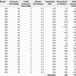
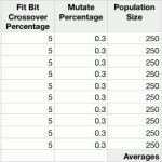
The attached Java implementation uses a mixture of crossover approaches. The crossover was initially programmed as only a random split crossover that occurred 65% of the time between two random, unweighted parents. Each pair of parents created one child for the next generation. At this point, it was possible to solve problems with a clause/variable ratio of 20-30 in under 20 minutes. Next step was to implement genetic mutation. In this algorithm, genetic mutations occur with equal probability in .3% of all bits. Mutation allowed for problems with a clause/variable ratio of 15 to be solved in under 20 minutes. At this point, the algorithm was not able to solve a problem with a clause/variable ratio of 10. I decided to try to implement a smarter crossover function that evaluates the fitness of each bit. I reverted my crossover function to use only the fit bit crossover, but performance was significantly decreased. I noticed that fit bit crossover would choose a lot of the same dominant bits and, as a result, the population became less diverse. Members began to look the same, generation after generation. For this reason, the fit bit crossover is only used 5% of the time. the other 60% of crossovers are done using random split crossover. Performance increased at this point. Still, the algorithm was unable to solve particularly hard problems (such as 50 variables with 275 clauses).
As another attempt at optimization, I decided that I would attempt to create two children from each set of parents and analyze their fitness. The child with higher fitness would be kept and the lower fitness child was thrown away. It seemed that this approach would give me a significant advantage. However, after implementing this feature, the algorithm could no longer solve problems with a clause variable ratio of 10 (such as 30 variables with 300 clauses). This feature was left out in the final implementation.
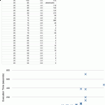
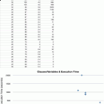
When collecting results, I noticed that there was a relation between the clause/variable ratio and the difficulty of a problem. In particular, the algorithm verified that as the clause/variable ratio approached 4.3, problems became virtually impossible for the algorithm to solve. One instance ran through over 100,000 generations of 1,000 members each without finding a solution. In this case, 5 of the 275 clauses were left unsolved by the population.
Find some variations on the tuning of the KSAT algorithm below. After some initial tests, the probabilities were solidified and further tests were done without change in the numbers.
Suggestions for Improvement
In particularly hard problems that ran for a significant time, it seems that the algorithm was stuck at a local maximum. I am wondering if introducing a random population member every so often will kick the algorithm in a new direction and possibly release it from the local maximum.
Instead of performing mutation with equal probability on each bit, I am wondering if a mutation should be performed on a per member basis instead. Perhaps we can see a performance increase if a member is chosen to be mutated. Once a member is found that should be mutated, choosing the least fit bit to mutate might prove advantageous.
Perhaps probabilities of certain mutations happening can fluctuate over time. It is possible that after a large number of generations, the algorithm requires some sort of change. Perhaps fluctuating population size with time will improve performance as well.
Conclusion
The KSAT algorithm implemented seems to have good performance as far as using BitSets for the data type as opposed to arrays. BitSets save time by doing fast comparisons. However, there may be memory issues as BitSets are mutable types and may be wasting space. Beyond implementation details like these, the algorithm seems to perform marginally. When compared to other algorithms, it seems like there must be better ways to solve KSAT problems. The algorithm was never able to solve problems such as 50 variables with 275 clauses (i.e. – 5.5 clause/variable ratio). In the future, I would write an additional program to help me analyze my results better in hopes of tuning probabilities more precisely. Regardless, through testing I was able to show that KSAT problems reach peak difficulty when the clause/variable ratio is near 4.3.
